

In this article, you will learn how to build a text clustering pipeline by combining large language model embeddings with HDBSCAN, a density-based clustering algorithm, to automatically discover topics in unlabeled text data.
Topics we will cover include:
- How to generate text embeddings for raw documents using a pre-trained sentence-transformers model.
- How to reduce the dimensionality of those embeddings with UMAP to prepare them for clustering.
- How to apply HDBSCAN to automatically discover topic clusters and visualize the results.
Clustering Unstructured Text with LLM Embeddings and HDBSCAN
Introduction
The current era of Generative AI seems to primarily focus on chat interfaces and prompts, but the range of applications of large language models, or LLMs for short, is not limited to just that. Indeed, one of their most powerful downstream abilities consists of turning raw, messy, unstructured text into semantically rich mathematical representations called embeddings. Once that’s done, we can use these text representations for a variety of machine learning use cases, with clustering being no exception.
In particular, embeddings can be combined with advanced, density-based clustering techniques like HDBSCAN, allowing as a result for the discovery of hidden topics, patterns, or categories in your collection of text documents: all without the need for prior labeling.
This article shows how to construct a text-based clustering pipeline from scratch. We will use a freely available dataset containing text instances, as well as an open-source LLM that has been trained for generating embeddings — i.e. a so-called embedding model. The icing on the cake: we’ll use free and handy, modern Python libraries providing implementations of clustering algorithms like HDBSCAN.
Step-by-Step Walkthrough
First, let’s start by installing the key Python libraries we will need:
- Sentence transformers, to load a pre-trained LLM for embedding generation from Hugging Face — you’ll need a Hugging Face API key, also called an access token, to be able to load the model.
- Umap-learn, to apply an algorithm to reduce the dimensionality of embeddings.
Likewise, if you are working on a local IDE instead of a cloud notebook environment and don’t have scikit-learn and pandas, you may need to install them too.
|
!pip install sentence–transformers umap–learn |
Now we start the coding part by getting some fresh data. The fetch_20newsgroups function, which fetches a dataset containing texts from categorized news articles, will do. Note that even though the dataset contains labels, we will omit them, as we are pretending not to know this information for the sake of clustering these data instances into groups based on similarity. Also, we sample down the dataset to 150 instances, which will be representative enough for our example.
|
import pandas as pd from sklearn.datasets import fetch_20newsgroups
# Fetching a highly targeted subset of data (~150-200 docs) categories = [‘sci.space’, ‘sci.med’, ‘rec.autos’] newsgroups = fetch_20newsgroups(subset=‘train’, categories=categories, remove=(‘headers’, ‘footers’, ‘quotes’))
# Sampling down into a representative, illustrative subset df = pd.DataFrame({‘text’: newsgroups.data, ‘true_label’: newsgroups.target}) df = df[df[‘text’].str.strip().str.len() > 100].sample(150, random_state=42).reset_index(drop=True)
print(f“Loaded {len(df)} text documents.”) print(“\nSample document:”) print(df[‘text’].iloc[0][:150] + “…”) |
Output:
|
Loaded 150 text documents.
Sample document:
Okay Mr. Dyer, we‘re properly impressed with your philosophical skills and ability to insult people. You’re a wonderful speaker and an adept politic... |
The next step is to obtain the embeddings from raw texts. To do this, we load all-MiniLM-L6-v2 from Hugging Face’s sentence-transformers library. This is a lightweight yet effective model to obtain embeddings quickly.
|
from sentence_transformers import SentenceTransformer
# Loading the free, open-source model model = SentenceTransformer(‘all-MiniLM-L6-v2’)
# Encoding text documents into dense vector embeddings print(“Generating embeddings…”) embeddings = model.encode(df[‘text’].tolist(), show_progress_bar=True)
print(f“Embedding matrix shape: {embeddings.shape}”) |
Since the embedding dimension is originally too high for clustering purposes, we now apply a dimensionality reduction technique by using the UMAP algorithm from the namesake library installed earlier:
|
import umap
# Reducing embedding dimensions to 5, to retain enough density information for clustering reducer = umap.UMAP(n_neighbors=15, n_components=5, min_dist=0.0, random_state=42) reduced_embeddings = reducer.fit_transform(embeddings)
print(f“Reduced matrix shape: {reduced_embeddings.shape}”) |
Now our numerical embedding vectors associated with news articles consist of five dimensions (attributes) only. Let’s see if this compact representation is meaningful enough to obtain insightful clustering by applying the HDBSCAN algorithm, which is a density-based clustering approach:
|
from sklearn.cluster import HDBSCAN
# Initializing HDBSCAN # min_cluster_size=8: we specified that each cluster must have at least 8 documents clusterer = HDBSCAN(min_cluster_size=8, min_samples=3, store_centers=‘centroid’) df[‘cluster’] = clusterer.fit_predict(reduced_embeddings)
# Counting instances per cluster cluster_counts = df[‘cluster’].value_counts() print(“\nCluster Distribution:”) print(cluster_counts) |
Important: the clustering results are partly influenced by the hyperparameter settings we defined for HDBSCAN. I recommend you try out other configurations for the minimum cluster size and other hyperparameters to explore how this affects results.
Result:
|
Cluster Distribution: cluster 0 101 1 49 Name: count, dtype: int64 |
It looks like HDBSCAN detected two clusters associated with high-density regions in the data space. Would there also be noisy points that were not allocated to either of these two clusters? Let’s check:
|
for cluster_id in sorted(df[‘cluster’].unique()): if cluster_id == –1: print(“\n=== CLUSTER: NOISE / UNCLASSIFIED ===”) else: print(f“\n=== CLUSTER: Discovered Topic #{cluster_id} ===”)
# Getting up to 3 sample texts from this cluster samples = df[df[‘cluster’] == cluster_id][‘text’].head(3).tolist() for i, sample in enumerate(samples, 1): clean_sample = ” “.join(sample.split())[:120] print(f” {i}. {clean_sample}…”) |
Output:
|
=== CLUSTER: Discovered Topic #0 === 1. Okay Mr. Dyer, we‘re properly impressed with your philosophical skills and ability to insult people. You’re a wonderful ... 2. I was at an interesting seminar at work (UK‘s R.A.L. Space Science Dept.) on this subject, specifically on a small-scale… 3. This is the second post which seems to be blurring the distinction between real disease caused by Candida albicans and t…
=== CLUSTER: Discovered Topic #1 === 1. It’s great that all these other cars can out–handle, out–corner, and out– accelerate an Integra. But, you‘ve got to ask ... 2. l diamond star cars (Talon/Eclipse/Laser) put out 190 hp in the turbo models, and 195 hp in the AWD turbo models, These ... 3. Sorry for the mis–spelling, but I forgot how to spell it after my series of exams and NO–on hand reference here. Is it s... |
Seems like all data points in the sample of 150 were allocated to either one of the two clusters identified, thus hinting at the clue that the news articles might easily separable according to topic.
For extra insight, we can show some cluster visualizations with the aid of the supplementary code provided below, which shows a scatterplot for every pairwise combination of the five existing components that describe each data point:
|
1 2 3 4 5 6 7 8 9 10 11 12 13 14 15 16 17 18 19 20 21 22 23 24 25 26 27 28 29 30 31 32 33 34 35 36 |
import matplotlib.pyplot as plt import seaborn as sns import itertools
# Creating a DataFrame for the 5 reduced embeddings and cluster labels reduced_df = pd.DataFrame(reduced_embeddings, columns=[f‘UMAP_D{i+1}’ for i in range(reduced_embeddings.shape[1])]) reduced_df[‘cluster’] = df[‘cluster’]
# Getting all unique pairwise combinations of the 5 dimensions dim_pairs = list(itertools.combinations(reduced_df.columns[:–1], 2))
num_plots = len(dim_pairs) num_cols = 3 num_rows = (num_plots + num_cols – 1) // num_cols
plt.figure(figsize=(num_cols * 5, num_rows * 4))
for i, (dim1, dim2) in enumerate(dim_pairs): plt.subplot(num_rows, num_cols, i + 1) sns.scatterplot( x=dim1, y=dim2, hue=‘cluster’, data=reduced_df, palette=‘viridis’, s=70, alpha=0.7, legend=‘full’ ) plt.title(f‘{dim1} vs {dim2}’) plt.xlabel(dim1) plt.ylabel(dim2) plt.grid(True, linestyle=‘–‘, alpha=0.6)
plt.tight_layout() plt.show() |
Result:
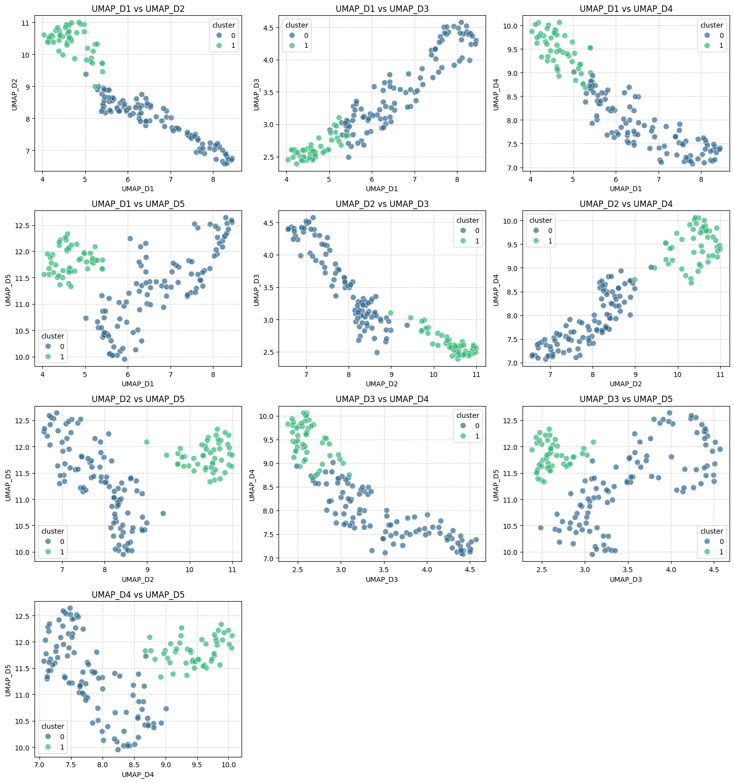
By trying different configurations for HDBSCAN, you may come across results in which the number of identified clusters could be different from two. Just give it a try!
Wrapping Up
Once we have gone through the process of building the text-based clustering pipeline, it is worth concluding by pointing out the key reasons why putting together LLM embeddings with HDBSCAN is worth it. These include the ability to retain and capture, to some extent, the true semantic meaning and linguistic nuances of the original text, thanks to the properties inherent to embeddings obtained through sentence-transformers. Moreover, HDBSCAN automatically determines an optimal number of clusters and is able to detect outlying points that might be noise or outliers that would distort group-level statistics.